Autonomous coding with local AI: is 8 GB of VRAM enough to run 30B models?
Can an 8 GB graphics card run local 26B, 30B, or even 35B models for autonomous coding? And how much do you gain by adding a second, 6 GB GPU bought for just over €100?
This test set out to answer that with real data.
This isn’t about asking a chatbot to write a program and copying the answer. Here the model works inside a coding agent: it receives a task, analyzes what it has to do, writes files, runs code, observes the results, fixes errors, and tries again until it completes the job or hits the established limits.
The test was run first using an 8 GB RTX 2080 SUPER. A 6 GB RTX 2060 was then added — a card that can be found on the used market for a bit over €100 — and the inference measurements were repeated to check what real improvement that second GPU brings.
The result is a lot more interesting than a simple VRAM bump: the extra 6 GB don’t turn the system into a single 14 GB GPU, but they can produce speed increases of roughly 39% to 98% depending on the model.
And for certain workloads, that changes the experience of using local AI quite a bit.
Quick results
Before getting into the technical part, here’s the headline data from the experiment:
| Test | Result |
|---|---|
| Starting GPU | RTX 2080 SUPER 8 GB |
| Second GPU | RTX 2060 6 GB |
| Total physical VRAM | 14 GB |
| CPU | Ryzen 7 5800X |
| RAM | 32 GiB |
| Main models | 26–35B, all MoE |
| Task | Autonomous coding in Python |
| Models that completed the task | 3 |
| Full runs | 2 per model |
| Inference improvement with the second GPU | +39% to +98% |
The second GPU wasn’t added to “make a specific model fit” and stop the test there. First it was checked what the system could do with 8 GB of VRAM, and only afterward was the performance change measured after adding another 6 GB.
1. Coding with a chatbot is not the same as coding with an agent
This difference is essential to understanding the results.
A chatbot can receive:
“Write me a wheel of fortune in Python.”
And return a block of code. That’s code generation.
A coding agent works differently:
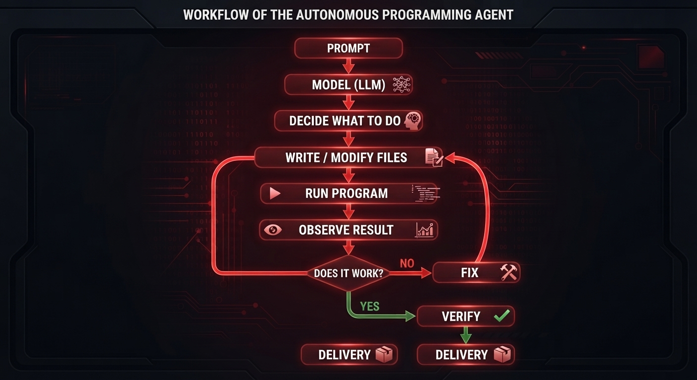
In this experiment, the model doesn’t work in isolation. The model is the reasoning component inside a system made up of:
- the AI model;
- OpenCode;
- Agente Jiménez;
- terminal tools;
- real project files;
- code execution;
- accumulated context;
- token limits;
- time limits.
That’s why the performance that matters here isn’t just how many tokens a GPU generates per second. What also matters is how many turns the agent needs to complete a task.
A model that generates 20 tokens/s but needs 40 iterations can take much longer than one that generates 15 tokens/s and solves the same task in six.
2. The hardware: 8 GB first, then 14 GB
The first part of the test is built around a very specific question:
How far can an 8 GB RTX 2080 SUPER go when used to run large local models in a coding agent?
The equipment used is:
| Component | Configuration |
|---|---|
| CPU | AMD Ryzen 7 5800X |
| RAM | 32 GiB |
| Main GPU | NVIDIA RTX 2080 SUPER, 8 GB |
| Additional GPU | NVIDIA RTX 2060, 6 GB |
| Total VRAM with both | 14 GB |
| Operating system | Garuda Linux + KDE Plasma |
| Inference engine | LM Studio / CUDA |
| Agent | Agente Jiménez |
| Coder | OpenCode |
| Test language | Python |
The main test focuses on the 8 GB RTX 2080 SUPER. Once those results were obtained, the 6 GB RTX 2060 was added and inference performance was measured again with the same models.
The idea is simple: 8 GB → measure → add 6 GB → measure again.
This way, the question of capacity can be separated from the question of performance.
3. How can an 8 GB GPU take part in running a 35B model?
At first glance it seems impossible. A 35-billion-parameter model quantized to Q4 can take up more than 20 GB on disk. The RTX 2080 SUPER used in this test only has 8 GB of VRAM.
The explanation is that the size of the model file doesn’t directly equal the amount of VRAM needed to process each token.
The model doesn’t fit entirely in the 8 GB of VRAM. Part of its weights and/or the structures needed for inference have to stay outside VRAM, in system memory, depending on the offload configuration.
Several factors come into play for the models used in this test:
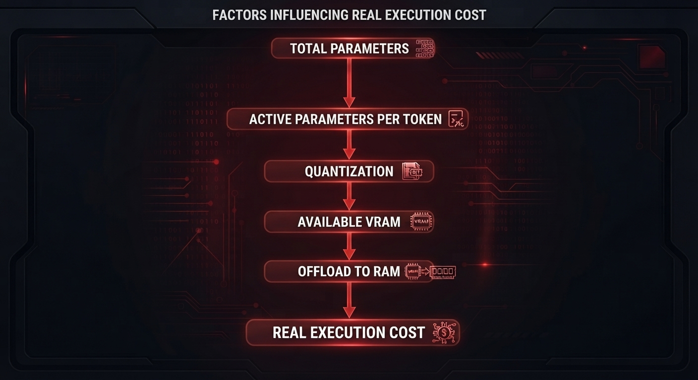
The three models that completed the test are Mixture of Experts (MoE) architectures. That means a model can have tens of billions of total parameters but activate only a portion of them for each token.
For example:
- 26B total → roughly 4B active;
- 35B total → roughly 3B active.
This radically changes the inference cost. A Dense 27B model, on the other hand, uses its parameters much more fully during each token.
Also, when part of the model doesn’t fit in VRAM, it can be kept in the system’s 32 GB of RAM. The problem is that RAM is vastly slower than a GPU’s memory.
On this machine, a real RAM bandwidth of roughly 23–33 GB/s was measured, which becomes one of the main bottlenecks whenever too much content has to come out of VRAM.
That’s why two models of similar size can behave in completely different ways.
4. The models used
These three models weren’t chosen for any special reason decided in advance. In the days before this test I individually tried more than a dozen different models on this same machine. Of all the ones that actually ran, these three seemed the most interesting to put through a full coding agent — they’re not “the best on the market” or a representative sample of anything; they’re simply the ones that, after that earlier screening, made the most sense to compare here.
Two concrete examples of why other candidates were left out: a variant quantized specifically for the ROCm/AMD engine wouldn’t even load on this machine (this setup uses the CUDA engine, which is incompatible with that packaging). Another, a 27B Whittle-MoE variant, did load and generate normally, but produced invented APIs (tk.Window, which doesn’t exist in Tkinter) and Spanish-language comments with corrupted words — likely due to quantization that was too aggressive for that model size.
The three models that completed the main test were:
| Model | Architecture | Parameters | Approx. active | Quantization | Size |
|---|---|---|---|---|---|
| cyber-tiel-coder-35b-a3b | MoE | 35B | ~3B | Q4_K_S | 21.8 GB |
| google/gemma-4-26b-a4b-qat | MoE | 25.2B | 3.8B | Q4_0 QAT | 15.6 GB |
| zai-org/glm-4.7-flash | MoE | 30B | — | Q4_K_M | 18.1 GB |
One important detail: the three models that made it to the end are MoE. Dense models around 27B were also tested, but none of them managed to complete the task under these conditions.
This doesn’t allow us to claim “MoE is always better than Dense.” What it does allow is something much more specific:
On this hardware, with this agent, these limits, and this task, the MoE models were the ones that managed to complete the autonomous coding cycle.
5. The task: a wheel of fortune
The chosen task is deliberately not a huge project. That’s precisely why it’s useful.
You don’t need a big project to put a coding agent to the test. Behind “a wheel of fortune with Tkinter” there are several small but real difficulties a model has to solve all at once, unaided:
- Animating without freezing the window. A smooth spin requires relying on the event loop itself (timers like
after()) instead of a plainsleep(), or the whole interface locks up while it spins. - A believable slowdown. It’s not enough to stop the wheel abruptly: the speed has to decrease gradually, frame by frame, with some braking factor.
- Correctly calculating the winning prize. Figuring out exactly which segment lands under the fixed pointer, based on the final spin angle, is modular arithmetic that’s easy to throw off by a whole segment with one sign or origin error.
- Fitting the text into each segment. Placing each spun prize’s name legibly inside its slice of the pie, without it running off or becoming unreadable.
- Managing the button’s state. Disabling it while spinning and re-enabling it when done, without it getting stuck if something goes wrong mid-animation.
- Staying within the standard library. All of this using only what Python ships with out of the box, no external dependencies, and delivering a program that genuinely runs as-is.
None of these difficulties is hard on its own. Together, and solved all at once with no human intervention, they’re enough to separate a model that “knows how to write Python” from one that also knows how to finish a program that actually works.
The agent was asked to create an application called ruleta.py, using Python and a native graphics library. The application had to include:
- a graphical window;
- a circular wheel;
- eight equal segments;
- different or alternating colors;
- the text of each prize;
- a fixed pointer;
- a “Spin the wheel” button;
- smooth animation;
- progressively decreasing speed;
- selection of the winning prize;
- presentation of the result;
- disabling the button during the spin;
- re-enabling it when finished.
The eight prizes were defined directly in the prompt. The prompt was the same for all the models. The request wasn’t adjusted to help any specific model. No manual corrections were made during the process either.
This is the exact, complete prompt as it was sent to the three models — copy it and try it yourself:
I want you to build a graphical application called ruleta.py.
Goal:
Create an interactive wheel of fortune with 8 AP-related prizes.

Functional requirements:

The application must open a window with a graphical interface.
The center must display a circular wheel divided into 8 equal segments.
Each segment must have a different or alternating color so they're easy to tell apart.
Each segment must display the text of a prize.
There must be a fixed indicator, like an arrow or pointer, that marks the winning prize when the wheel stops.
There must be a visible button with the text "Spin the wheel."
When the button is pressed:
The wheel must start spinning.
It must do so with a smooth animation.
The speed must decrease progressively.
It must eventually stop on one of the 8 prizes.
When the wheel stops, the winning prize must be clearly displayed on screen.
While the wheel is spinning, the button must be disabled to prevent repeated clicks.
When the spin ends, the button must be re-enabled.

Wheel prizes:

"You win a browser privacy audit"
"You win access to the worldwide SDR receiver map"
"You win a tutorial for creating your first local AI"
"You win a guide to listening to SDR radio from scratch"
"You win an analysis of your online digital footprint"
"You win access to radio and signal tools"
"You win a guide to protecting your digital identity"
"You win exclusive resources from the Acuántico Power lab"

Use Python as the main language.
Use a native Python graphics library.
The code should be organized, readable, and have useful comments.
Avoid unnecessary dependencies.
The wheel must work without an internet connection.
If the project needs several files, create them with a clean structure.
Include clear instructions for running the program.
The purpose was to check how each model behaved when faced with a small but complete task: create, run, check, and finish.
It also tests real geometry, not just program logic: dividing a circle into 8 exactly equal slices, calculating the angle of each one, and rotating each prize’s text so it follows the orientation of its slice are concrete trigonometric calculations, not a template that can be copied without understanding it. On top of that there’s the full visual effect that has to be pulled off: the wheel has to spin, you have to be able to see it progressively losing speed until it stops — not stopping abruptly — and the prize text has to rotate glued to the wheel at all times, not fixed on screen. It’s the part of the prompt that’s easiest to describe badly or oversimplify, and where it shows most clearly whether a model actually understood the task or just generated something that resembles it.
It’s also no accident which task wasn’t chosen. I deliberately didn’t ask for a Tetris or a Snake or any other classic of that sort. That kind of project shows up so often in these models’ training — precisely because they’re the typical examples used to measure and optimize scores on the most common coding benchmarks — that a model can solve them well without that proving much: it could be reproducing something memorized, not reasoning through the task from scratch. A wheel with made-up prizes and a prompt written specifically for this test reduces that advantage and brings the result closer to what would happen with any real assignment that hasn’t already been solved a thousand times on the internet.
6. The same task, with one GPU and with two
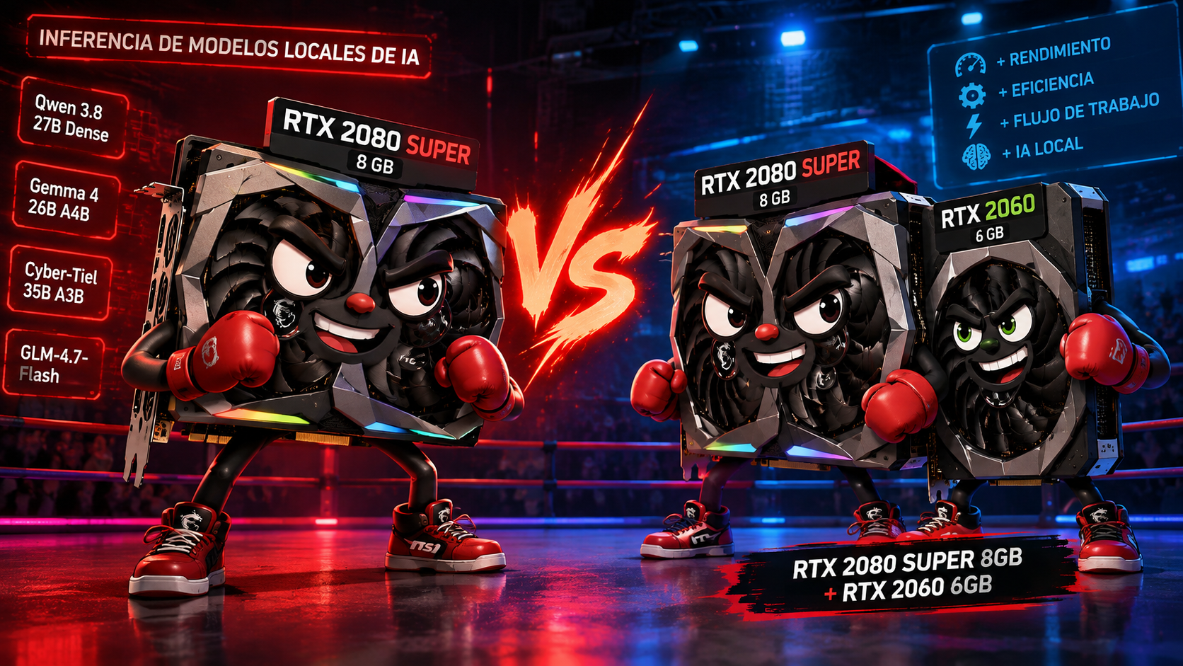
Each of the three main models completed the task twice, but not under the same conditions: the first time using only the RTX 2080 SUPER, the second time with the RTX 2060 already installed alongside it. Unlike the raw-inference comparison in sections 9 through 15, this is the comparison at the level that actually matters for an autonomous agent: the full pipeline, start to finish, with one GPU and with two.
The results were:
Before reading the table: the Tok/s figures below aren’t comparable to the improvement percentages in sections 10-15. These are two different measurements — this one is the average inside a full agent run, that one is direct inference — and the reason they don’t line up is explained further down.
| Model | Run | Verified | Time | Iterations | Tokens | Tok/s |
|---|---|---|---|---|---|---|
| Cyber-Tiel 35B | 1 (2080S only) | Yes | 38.1 min | 30 | 21,627 | 10.27 |
| Cyber-Tiel 35B | 2 (2080S+2060) | Yes | 42.4 min | 41 | 21,994 | 12.97 |
| Gemma 4 26B | 1 (2080S only) | Yes | 13.3 min | 14 | 10,628 | 15.14 |
| Gemma 4 26B | 2 (2080S+2060) | Yes | 4.2 min | 6 | 3,010 | 17.03 |
| GLM-4.7-Flash | 1 (2080S only) | No | 90.5 min | 49 | 26,751 | 4.69 |
| GLM-4.7-Flash | 2 (2080S+2060) | No | 90.3 min | 97 | 36,207 | 4.19 |
The iterations are real generation calls logged by LM Studio. They’re not estimates. There were also no extra rounds of visual repair in any of the six runs.
Since this is a single run per configuration, this table doesn’t allow for claims about statistical consistency. It’s useful for seeing the effect of the second GPU on the full task, not for measuring how much a model varies between identical attempts.
Note on the Tok/s column: it’s the average of the per-call generation speeds logged by LM Studio, not the result of dividing total tokens by total run time (which includes context reprocessing between iterations).
7. What these results actually show
Gemma 4 26B: very fast, with or without the second GPU
Gemma was, in both configurations, the model that needed the least time. With the RTX 2080 SUPER alone it took about 13 minutes and 14 iterations; with the RTX 2060 added, that dropped to a bit over 4 minutes and only 6 iterations. That’s a considerable difference — but with only one run per configuration, there’s no way to know for certain how much of that comes from having the second GPU available and how much is normal variability between attempts for this particular model.
What is a clean data point: the per-call generation speed barely changed (15.14 → 17.03 tok/s). Total time didn’t depend mainly on generating faster, but on the number of turns the agent needed to close out the task.
This shows something important about agents: generation speed alone doesn’t determine completion speed.
Cyber-Tiel 35B: faster per call, but not faster overall
Cyber-Tiel needed considerably more time than Gemma in both configurations: 38.1 minutes with just the 2080 SUPER, 42.4 minutes with the 2060 added. The result is counterintuitive: with the second GPU, per-call generation speed went up (10.27 → 12.97 tok/s), but total task time was higher, not lower, because that run needed more iterations (41 vs. 30) for a similar volume of generation (21,994 vs. 21,627 tokens). The pipeline verified the result both times.
This confirms, with an even clearer example, that generation volume and completion time shouldn’t be collapsed into a single speed metric: more tokens per second doesn’t guarantee finishing sooner. With only one run per configuration, we still can’t talk about statistical consistency.
GLM-4.7-Flash: the problem was closing the loop, with and without the second GPU
GLM is especially interesting. It took roughly 90 minutes in both configurations — 90.5 minutes with just the 2080 SUPER, 90.3 minutes with the 2060 added — with the second GPU not changing the conclusion: the pipeline never managed to close the loop in either run. And yet the generated program was functional both times. The problem wasn’t simply “it doesn’t know how to code.” The problem was in the agent’s behavior.
In neither configuration did the pipeline manage to properly close the loop within its own limits. There were:
- 49 iterations with just the 2080 SUPER;
- 97 with the 2060 added — almost double, in practically the same total time, consistent with the inference-speed improvement measured for this model in section 10;
- 0 natural completions (the model never reached a stopping point on its own) across the 146 combined iterations.
This matters because it shows a distinction that usually gets lost in traditional benchmarks: a model can produce valid code and still not behave correctly inside an autonomous agent — and a faster GPU doesn’t fix that problem, it just lets it try more times without succeeding.
Looking through the logs of one of the runs offers a clue as to why closing the loop was so hard: of the recorded edit calls, 19 were on ruleta.py itself and 18 were on the test file the model decided to create on its own — almost a 50/50 split. A good chunk of the effort went into rewriting its own tests on every turn, not just fixing the program; a pattern consistent with chasing its own tail (adjusting the test to the code, touching the code, breaking the test) instead of converging on a version that satisfied both at once.
With just the 2080 SUPER there was also a failure unlike anything else seen in this test: after 39 minutes of real progress — files written, tests running, errors fixed — the connection to the inference engine cut out abruptly, with no prior error in the logs. With both GPUs this never happened in any run. There’s no way to confirm the cause with the available data: it could be memory pressure, a one-off CUDA fault, a client-server connection timeout, or some other combination, and without driver logs from the exact moment of the drop, causality can’t be pinned down with certainty.
Hypothesis, unconfirmed: with an 18 GB model squeezing an 8 GB card, memory pressure is the most reasonable explanation — one more warning for anyone considering a single-GPU setup with large models: it can not only be slower, it can also be less stable.
For autonomous coding, knowing when to keep going and when to stop is also part of the problem.
8. The generated code: it’s not enough for the agent to say “verified”
The verified status needs to be read carefully. It means the pipeline managed to complete its verification mechanism. It doesn’t mean the program is perfect.
That’s why the result also needs to be evaluated from the perspective of the generated program. All three models produced a functional wheel with the fundamental requested elements.
Technical note: a pipeline bug can look like a model failure
During this investigation a real bug was found and fixed in the pipeline itself, and it’s worth mentioning because it changes how you should read a “not verified” result. The token budget for each call is split between what the model can generate as a response and what it can receive as input context. An initial configuration reserved too much for the former: out of a 29,952-token context, 20,480 were set aside for output, leaving only about 9,500 for input — less than a single typical retry of this pipeline takes up (~15,000 tokens, between the current file and the verification report). The result was that several retries failed on their very first turn, before the model could even see why the previous one had failed — something that, seen from the outside, looks a lot like “the model isn’t up to the task.”
This doesn’t change any of the results published in this article — it was fixed before the runs that make up this comparison — but it’s a useful reminder: when a local model doesn’t converge inside an autonomous agent, it’s worth checking the pipeline first before concluding the model is the problem.
Cyber-Tiel
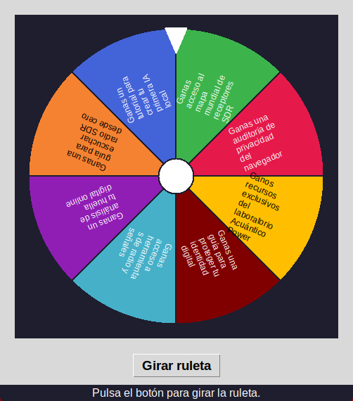
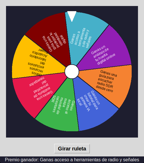
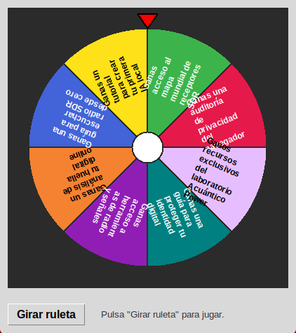
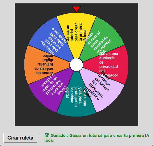
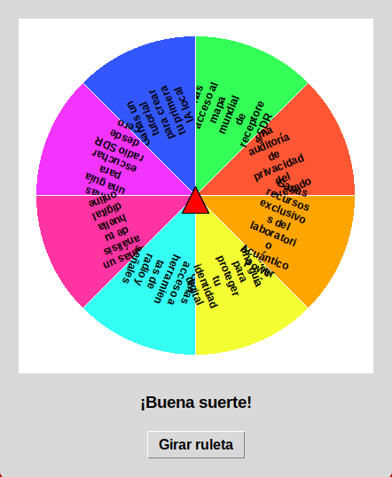
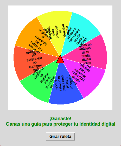
The implementation uses a RuletaFortuna class, draws the segments with create_arc, and uses root.after() to run the animation without blocking the interface. It also includes a deceleration factor of roughly 0.985 and a dedicated function to adapt text contrast based on the background.
I found a small transcription error in one of the prizes: it reads “Ganos” where the prompt said “Ganas” (“You win,” in Spanish). It’s a minor slip, but it shows why checking the result still matters even when the agent declares it’s done.
Real screenshot — Run 1 (2080S only):
Real screenshot — Run 2 (2080S+2060):
Gemma 4
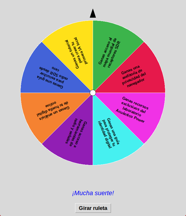
It uses a very similar strategy: segments via pieslice, animation via after(), progressive deceleration, graphical interface, spin button, prize selection.
The prizes are correctly transcribed. Its implementation is simpler and doesn’t include the contrast logic used by Cyber-Tiel.
Real screenshot — Run 1 (2080S only):
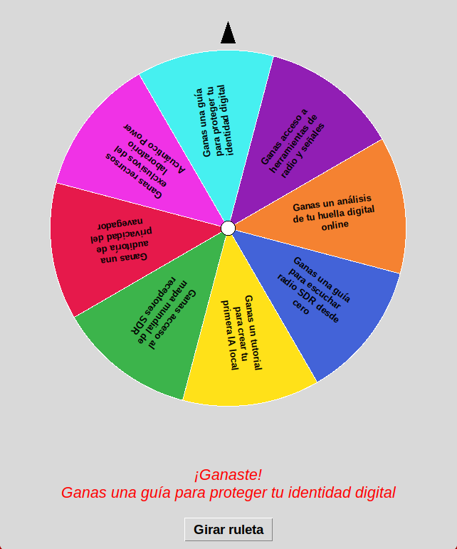
Real screenshot — Run 2 (2080S+2060):
GLM-4.7-Flash
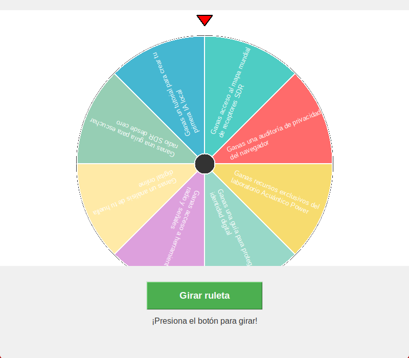
Its program also turned out functional. The structure separates widget creation from drawing the wheel and keeps a reasonably organized graphical interface.
What’s interesting is that the code worked even though the agent couldn’t successfully finish the verification process. This again shows that “not verified” and “broken code” aren’t synonyms.
Real screenshot — Run 1 (2080S only):
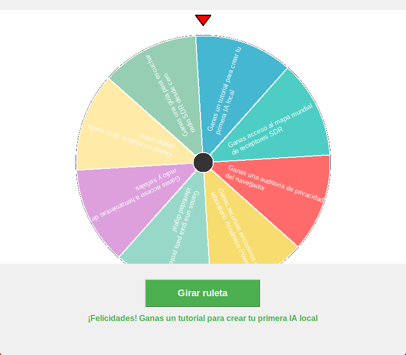
Real screenshot — Run 2 (2080S+2060):
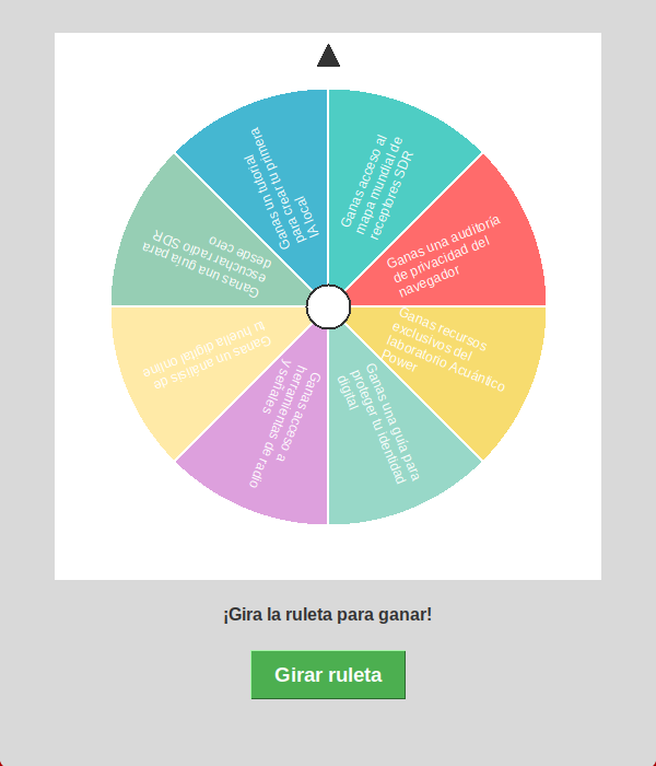
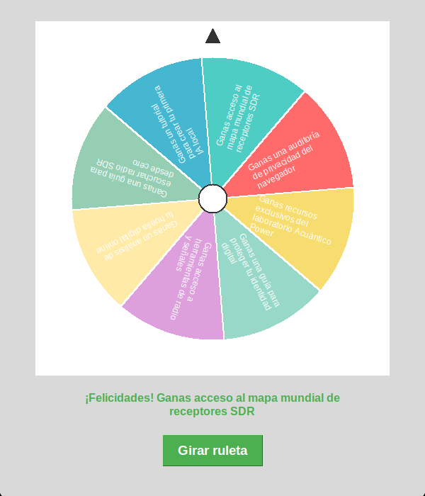
9. The second GPU: the test that actually matters
So far we have an 8 GB RTX 2080 SUPER as a baseline. The next question is much more practical: what happens if we add a second, cheap graphics card?
The card chosen was a 6 GB RTX 2060. The goal wasn’t to build a thousand-euro workstation. The idea was much simpler:
Can a used GPU costing a bit over €100 make a noticeable difference to a system that already has an RTX 2080 SUPER?
To check this, inference was measured directly with LM Studio before and after adding the RTX 2060. The same models were used for this second measurement.
10. RTX 2080 SUPER vs. RTX 2080 SUPER + RTX 2060
The results are clear:
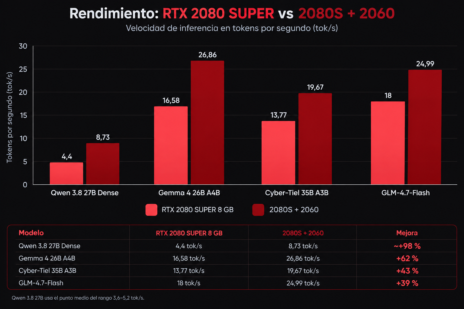
This is one of the most interesting results of the whole experiment. The second GPU does bring a noticeable improvement. But how much depends heavily on the model’s architecture.
11. How much difference does a 6 GB RTX 2060 really make?
In terms of tokens per second, the answer is: quite a lot.
We’re not talking about a 5% or 10% bump. The MoE models used in this test improved by 39% to 62%. The 27B Dense model roughly doubled its speed: 3.6–5.2 tok/s → 8.73 tok/s. That’s an improvement of up to roughly 98%.
But it’s worth understanding why. With a single 8 GB RTX 2080 SUPER, a large Dense model depends much more heavily on offloading to RAM. When another 6 GB of VRAM is added, a much larger portion of the model can stay in GPU memory. The bottleneck shifts.
RAM no longer has to be involved as much in moving the data needed to generate each token. That’s why the Dense model is precisely the one that shows the biggest relative jump.
12. And what happens with the MoE models?
Here the situation changes. MoE models already behave relatively well with little VRAM, because the number of active parameters per token is much smaller than the total number of parameters. That’s why the jump from adding the RTX 2060 is more modest:
- Gemma 4: +62%
- Cyber-Tiel: +43%
- GLM: +39%
But “more modest” doesn’t mean small. A 39% increase means going from roughly 17–19 tok/s → 24.99 tok/s. Over a long generation session, that difference adds up. And in an agent doing dozens of iterations, it can have a substantial impact.
13. Does 14 GB of VRAM really mean 14 GB?
Not exactly. This matters for anyone considering putting together a similar setup.
Two cards with 8 GB and 6 GB don’t turn into a single virtual 14 GB GPU with the same characteristics as an actual 14 GB card. The memory is still physically split across two devices. The software has to split the work.
In this case, LM Studio lets you use both GPUs, but that split doesn’t amount to having a single, unified VRAM pool.
So the correct way to describe this configuration is: 8 GB RTX 2080 SUPER + 6 GB RTX 2060 with distributed execution, not “a 14 GB GPU.”
14. The size of the second GPU matters less than it seems
There’s another interesting conclusion. The second card doesn’t need to be as powerful as the main one to be useful.
The RTX 2060 has 6 GB of VRAM, less power than the RTX 2080 SUPER (same Turing process, but a smaller chip with fewer cores), and a much lower used-market price. In this configuration, LM Studio distributed the model’s load across both GPUs: the second card doesn’t act as a transparent extension of the first one’s VRAM — each GPU keeps its own memory, and it’s the backend that decides how to split the model and the workload between devices. Even so, that split reduces the dependency on system RAM.
The measured result shows that a relatively cheap secondary GPU can have a significant effect on local inference. That doesn’t mean any combination of GPUs will produce the same numbers. It will depend on: architecture, model size, quantization, how the load is split across devices, bandwidth, CPU, RAM, context, and the software used.
But the principle is demonstrated on this machine.
15. Is it worth buying a cheap second GPU?
With the data from this test, there’s a fairly clear answer: if you already have a compatible GPU and can get a cheap second card, the improvement can be genuinely noticeable.
The RTX 2060 used here costs a bit over €100 on the used market. For that outlay, the measurements obtained were:
- up to +98% on a Dense 27B;
- +62% on Gemma 4;
- +43% on Cyber-Tiel;
- +39% on GLM.
That’s not a theoretical improvement. It’s a measured difference in tokens per second.
That said, there’s an important distinction between economic value and technical compatibility. A second GPU means more power draw, more heat, more space taken up, more complexity, a motherboard and power supply that can handle it, and software capable of correctly distributing the model.
So it doesn’t make sense to buy a second GPU purely because it adds 6 GB. It makes sense when those 6 GB address a real bottleneck. In this experiment, that bottleneck was especially clear in the large, dense models.
16. Raw inference vs. autonomous coding
There’s a wrong conclusion to avoid here. The second-GPU numbers are inference tokens per second, not a promise that a coding task will take exactly 39%, 62%, or 98% less time.
The agent has an additional cost. Every iteration involves: receiving the context, processing it, generating a response, running tools, reading the results, folding that result back into the context, and inferring again. And the context keeps growing.
In GLM’s case, for example, the sum of tokens sent across the prompts of its 97 iterations reached roughly 1.77 million tokens. That doesn’t mean the model had 1.77 million tokens inside a single context window: those are tokens accumulated across successive calls, not a simultaneous context. That’s why the 17–27 tok/s from the direct measurements don’t translate directly into the 10–17 tok/s observed during autonomous coding. The agent is doing a lot more than generating text.
This distinction is essential when comparing GPUs for local agents.
The inference benchmark tells you how much faster the engine can go. The agent benchmark tells you how much faster a real task can go.
17. Dense vs. MoE: here’s the difference
One of the clearest conclusions from this test is that you shouldn’t look only at the parameter count. A 27B Dense model can turn out to be much more demanding than a 35B MoE. Why?
35B MoE
→ ~3B active per token

27B Dense
→ most of its 27B take part in every token
This doesn’t mean the inactive parameters are irrelevant for memory. They’re still part of the model. But it does massively change the computational cost of generating each token. The inference measurements reflect that:
| Model type | Approximate performance |
|---|---|
| Dense 27B with 8 GB | ~2.3–5.5 tok/s |
| MoE 26–35B with 8 GB | ~13–19 tok/s |
The “Dense 27B with 8 GB” range aggregates the broader set of ~27B Dense candidates tested on this machine, not just the specific Qwen 3.8 27B Dense measurement from section 10 (3.6–5.2 tok/s), which corresponds specifically to the with/without second-GPU comparison tests.
Architecture can matter as much as, or more than, a model’s nominal size.
18. And what about the 27B Dense models?
In this test, the roughly 27B Dense models didn’t manage to complete the autonomous coding task. This deserves an explanation, because it would be easy to blame it entirely on the 8 GB of VRAM.
The logs show the problem was also related to the models’ own behavior. One of the candidates tended to keep excessively long reasoning chains and repeatedly exhausted its output budget. Another showed generation behavior poorly suited to the agent’s time limit.
So the correct takeaway isn’t: “27B Dense doesn’t work with 8 GB.”
The 27B Dense models tested in this experiment didn’t manage to complete the task under these conditions.
That’s an important distinction. The hardware is only one part of the system.
A concrete case: three variants of the same model, three attempted fixes
One of the 27B Dense candidates was tried in three different quantizations over the course of this investigation, each one after diagnosing why the previous attempt had failed. It’s worth detailing because it illustrates the underlying problem well.
The first quantization (very aggressive, ~3.7 bits per parameter) kept running out without writing a single file, burning through its reasoning budget without ever invoking a tool. The second, closer to the original model (Q4_K_M, 17.7 GB), reasoned normally in isolated tests, but didn’t fit in this machine’s combined VRAM and its speed suffered. The third (Q3_K_M, 14.3 GB) did fit and got close to 10 tok/s — but, faced with this task’s real prompt, it fell into the same problem as the first: with the lowest available reasoning setting (“low”), it spent 15,972 of a 16,000-token budget thinking, without writing a single character of code; with reasoning fully disabled (“none”) it spent 7,942 of 8,000 doing the same thing.
The most telling part is the contrast: that same model, faced with a simple test prompt (a class with a button that increments a counter), responded in just over three minutes using barely 80 reasoning tokens. Faced with this article’s actual task — with animation, geometry, and a test suite to satisfy — the same setting that worked perfectly on the simple test wasn’t enough for the model to know when to stop thinking.
Speeding it up with a draft model (speculative decoding) from the same family was also tried, hoping to break through its speed ceiling — the load failed outright due to lack of VRAM for the draft cache, without even enough headroom to test it.
No reasoning setting tested — low, none, or the default — avoided the problem on the real task. That’s why these Dense candidates were left out of the final comparison: not because of the model’s size or the available VRAM, but because they didn’t know when to stop reasoning in front of a sufficiently complex task.
19. The hidden cost of context
When talking about running local models, a lot of attention usually goes to parameters, VRAM, and tokens per second. In autonomous agents there’s another factor that can be even more important: context.
Every new iteration can add executed commands, results, messages, file contents, errors, fixes, and previous instructions. So a task that starts with a small prompt can end up forcing the model to process a huge amount of context.
This explains why a model can perform excellently on a short-prompt benchmark and then behave much more slowly inside an agent. In this sense, autonomous coding is a far more demanding test than a normal conversation.
20. What this test actually shows
After running these tests, the most useful conclusions are fairly concrete.
An 8 GB RTX 2080 SUPER can be used for autonomous coding with large models
With quantization, MoE, and RAM offload, it’s possible to work with 26–35B models. That doesn’t mean every model of that size behaves the same way. Architecture matters enormously.
MoE models have a clear advantage in this scenario
The three models that completed the task are MoE and use roughly 3–4B of active parameters per token.
A cheap second GPU can add quite a lot
Adding a 6 GB RTX 2060 produced improvements of between +39% and +98% in the inference tests carried out.
The benefit is especially interesting for Dense models
The 27B Dense model improved the most in relative terms, going from roughly 3.6–5.2 tok/s to 8.73 tok/s.
Speed is not the same as the ability to finish
Gemma was extremely fast on the first run. GLM, on the other hand, produced a functional program but spent around 90 minutes without properly closing the process. In an autonomous agent, the ability to finish is part of the performance.
What this test does and doesn’t prove
Summarizing all of the above in one place, so it’s clear how far these conclusions go and where extrapolation should stop:
| This test does prove | This test doesn’t prove |
|---|---|
| That these models could run on this machine | That any 35B model works with 8 GB |
| That all three models produced a functional application | That all three agents correctly completed the loop |
| That the second GPU increased measured performance | That any pair of GPUs scales the same way |
| That the MoE models tested behaved favorably | That MoE is always superior to Dense |
| That a 2060 can add extra performance | That a second GPU is always the better economic choice |
| That tok/s and task completion are different metrics | That +98% tok/s means +98% productivity |
| That offload allows working with models bigger than VRAM | That the whole model fits in 8 GB |
21. Limitations of this test
These results need to be read within their conditions. This isn’t a universal benchmark of coding models. The main limitations are:
- A single main task. The wheel doesn’t represent large projects, backends, databases, or complex applications.
- A single run per GPU configuration. The 2080S-only / 2080S+2060 comparison in section 6 has exactly one case per side — useful for seeing the effect on the full task, not for talking about statistical consistency.
- Two different GPU comparisons, with different goals. Sections 9 through 15 measure raw inference (tokens per second) with several measurements per model. Section 6 measures the full agent pipeline, but with only one run per configuration — use it to see the qualitative effect, not as an isolated inference-speed measurement.
- The results depend on the whole stack. Model, quantization, LM Studio, OpenCode, Agente Jiménez, CPU, RAM, and GPU configuration are all part of the result.
- Not every Dense model completed the task. So there isn’t a balanced Dense-vs-MoE comparison here in terms of completion time for the same task.
- Multi-GPU splitting depends on the software. Physically having 14 GB isn’t the same as having a single GPU with 14 GB of unified memory.
These limitations don’t invalidate the experiment. They define which questions it can answer.
22. Configuration to reproduce the test
| Parameter | Value |
|---|---|
| CPU | Ryzen 7 5800X |
| RAM | 32 GiB |
| GPU | RTX 2080 SUPER 8 GB |
| Second GPU | RTX 2060 6 GB |
| System | Garuda Linux + KDE Plasma |
| Engine | LM Studio + CUDA |
| GPU split | --gpu 0.5 (see note) |
| Agent | Agente Jiménez |
| Coder | OpenCode |
| max_output_tokens | 8192 per call |
| pipeline_task_timeout_seconds | 7200 per case |
| Task | ruleta.py in Python |
| Prompt | identical across models |
The test was run using the CUDA engine. On this machine, the Vulkan backend wasn’t used due to stability issues.
Note on the GPU split: LM Studio exposes no fine-grained multi-GPU control (no tensor-split, no main-gpu, no device selector in the interface or in the per-model persisted config). The only available parameter is a coarse ratio flag — --gpu max or intermediate values like --gpu 0.5 — and the engine itself decides internally how much goes to each card. This test used --gpu 0.5 for all three models, confirmed as the configuration that loaded reliably without a VRAM allocation error; it wasn’t possible to verify the exact per-GPU split with nvidia-smi for each of the six runs individually. This limits how precisely the experiment can be reproduced with other software that does expose that control.
23. So, is a second GPU worth it?
If the question is purely whether an extra 6 GB from a cheap RTX 2060 can make a real difference, this experiment’s numbers say yes. The measured increase wasn’t marginal: +39%, +43%, +62%, and up to +98%.
But the second GPU shouldn’t be seen as a cheap substitute for a modern, high-VRAM GPU. It’s a different strategy.
If you already have an RTX 2080 SUPER and want to experiment with local AI, a used RTX 2060 can make sense, because it lets you increase the available processing capacity without having to replace the main card.
On the other hand, if you’re starting from scratch, you need to compare the total cost of: one large GPU, two used GPUs, power draw, power supply, cooling, and software compatibility.
The test shows that a dual-GPU setup works and can meaningfully speed up inference. It doesn’t show that it’s always the economically optimal choice for every user.
24. The most important conclusion
The most interesting part of this experiment isn’t really the wheel. It’s what happens when you combine large models, old hardware, and autonomous agents.
An 8 GB RTX 2080 SUPER — a card that no longer belongs to the current generation — can take part in a system capable of running local 26–35B models and completing autonomous coding tasks.
The secret isn’t any single feature. It’s the combination: quantization + MoE + active parameters + RAM + inference software + agent + tools.
Then, adding a 6 GB RTX 2060 for a bit over €100 doesn’t magically turn the machine into a unified 14 GB VRAM box. But the measurements show something more useful: those extra 6 GB can significantly reduce the bottleneck and boost inference speed by between 39% and 98% depending on the model.
For a large Dense model, the difference can come close to doubling. For MoE models, the increase is smaller, but still big enough to notice.
And that’s probably the most useful lesson for anyone wanting to build a local AI lab with used hardware:
You don’t always need to buy an expensive new GPU. Sometimes, understanding where the bottleneck actually is lets you get a lot more out of the hardware you already have.
25. Production test: when we want a finished result
The benchmark ended here. Everything measured so far — times, iterations, verifications, tok/s — describes what a local model can complete inside an autonomous agent, with a limited number of attempts and no human intervention during the task.
Now we’re using one of the models from the experiment in a completely different workflow: collaborative, with several rounds of requests and corrections, just like you’d work with any tool day to day — not another measurement of the same benchmark.
As a closing example of that: Gemma 4 26B (the fastest and most balanced of the three models in this comparison), running solely on the 8 GB RTX 2080 SUPER, was asked to analyze the six real wheel implementations generated during the benchmark — from the three models, with and without the second GPU — and keep the best ideas from each to build a new version meant for the web: self-contained HTML, CSS, and JavaScript, with a professional finish, and with the 8 prizes turned into real links to other articles from this lab.
It took several rounds of specific requests — matching the color palette to this site’s, keeping the prize text from overlapping, giving the finish more depth — before reaching a version that genuinely worked well. That’s what working with a local model in a real workflow actually looks like: not a single perfect attempt, but refining it with increasingly specific instructions until the result comes together.
Try it yourself — spin the wheel, and each prize takes you to a related article from this lab.
Frequently asked questions
Can you run a 30B model on an 8 GB RTX 2080 SUPER?
Yes, at least with the MoE models tested in this experiment. The combination of quantization, active parameters, and RAM offload makes it possible to run models whose total size is well beyond the 8 GB of VRAM available.
Does a 6 GB RTX 2060 actually help an RTX 2080 SUPER?
Yes. In the measurements taken, combining both GPUs increased inference speed by roughly 39% to 98%, depending on the model.
Do 8 + 6 GB become 14 GB of VRAM?
No. The two cards keep their own memory. The software can split the model and the workload between them, but they don’t behave exactly like a single GPU with 14 GB of unified VRAM.
Which model was fastest at autonomous coding?
Gemma 4 26B needed the least time in both runs, although it showed significant variation between the two: roughly 4 and 13 minutes.
Which model was most consistent?
Cyber-Tiel 35B produced verified results in both runs, with roughly 38–42 minutes of total time and around 22,000 tokens generated each time.
Did GLM-4.7-Flash fail?
Not exactly. The generated program turned out functional, but the pipeline failed to automatically close the verification process in either run. The problem was in the autonomous loop, not simply in the code produced.
Is MoE always better than Dense?
No. This experiment doesn’t let us establish a universal rule. What it does show is that the MoE models tested were the ones that managed to complete the task under these conditions.
What are active parameters?
They’re the parameters involved in processing each token in an MoE architecture. A model can have 35B total parameters and only activate a fraction of them for each token.
Can a local AI code without human intervention?
In this test, the three models that reached the final result left behind a functional application with no human intervention during the task. In two cases, the pipeline itself also automatically confirmed the result.
Why is agent performance lower than a tokens-per-second benchmark?
Because an agent doesn’t just generate tokens. It has to process the accumulated context, run commands, read results, and reason again. The more iterations it runs, the higher the context cost can get.
What does OpenCode actually add compared to a chatbot?
OpenCode lets you work on real files, run commands, and observe the results within the project. The model can use that information to decide what to do next. A conventional chatbot is mainly limited to generating a text reply.